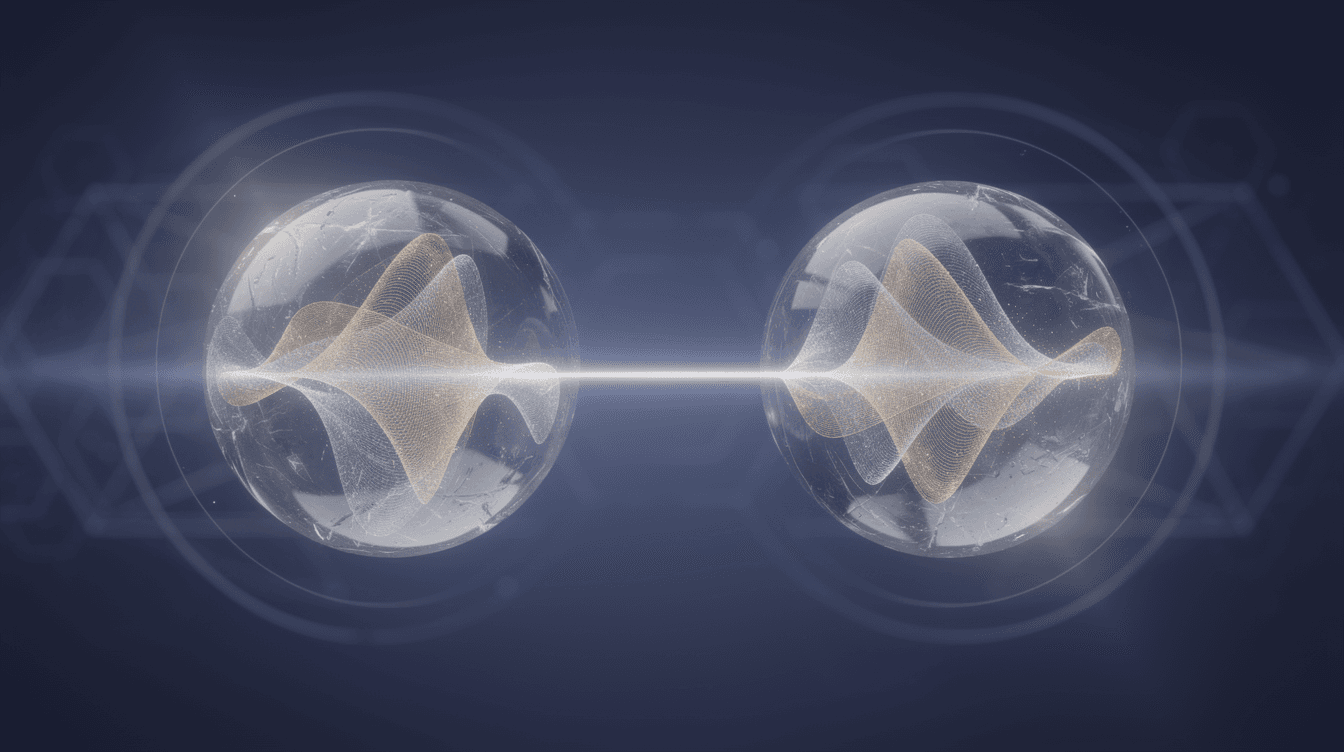
The Quest for Identifiable World Models
To plan and reason, an AI must distill high-dimensional observations—pixels from a camera, sensor readings—into a compact world model that captures the true hidden state.
A fundamental challenge is identifiability: can the learned representation recover the underlying latent variables up to simple, harmless transformations?
Many self-supervised methods fail to guarantee this, allowing representations that are scrambled or distorted.
The paper introduces a remarkable property: linear identifiability.
It means the learned latent code equals the true latent state rotated by an orthogonal matrix—information is perfectly preserved in a linearly invertible way.
And it shows that a learner called LeJEPA (alignment plus Gaussian regularization) achieves this property, but only when the world’s latents follow a Gaussian distribution.
This “if and only if” theorem reshapes how we think about the role of statistical assumptions in representation learning.
How LeJEPA Learns the World
The world is a dynamical system: a latent state ( z ) evolves under stationary, additive-noise dynamics ( z' = m(z) + \eta ), and we observe it through an unknown nonlinear mapping ( x = g(z) ).
LeJEPA trains an encoder ( h ) that maps each observation to an embedding.
It balances two objectives:
- Alignment: minimize the expected squared distance ( | h(z') - h(z) |^2 ) for consecutive states, encouraging temporal coherence.
- Gaussianity constraint: the distribution of embeddings must be standard normal ( \mathcal{N}(0, I_n) ), enforced by the Sketched Isotropic Gaussian Regularizer (SIGReg).
This combination is subtle and powerful.
The alignment term pushes the encoder to preserve what is stable across time, while the Gaussianity constraint provides a fixed statistical anchor that forbids nonlinear distortions.
Together they force the encoder to become a linear, orthogonal map—a pure rotation of the true latents.

The Gaussian Secret: Why a Bell Curve Unlocks Linear Recovery
At the heart of the forward theorem lies a spectral argument using Hermite polynomials, the natural basis for functions under a Gaussian measure.
Any candidate encoder ( h ) can be expanded in Hermite polynomials.
When the true latents are Gaussian, the alignment loss decomposes into a sum of terms, each associated with a polynomial degree.
Crucially, the coefficient for the linear degree is larger than for any higher-order degree.
Nonlinear components contribute less to temporal correlation and are thus strictly penalized.
Minimizing alignment while staying Gaussian forces all nonlinear contributions to vanish.
What remains is a linear map, and the Gaussian constraint fixes its covariance to identity, making it an orthogonal transformation ( Q ).
So the learned representation is exactly ( h(z) = Qz ), a rotated version of the truth.
This is Theorem 1: if the world is Gaussian, LeJEPA linearly identifies the latents.
The Flip Side: Non-Gaussian Worlds Break the Guarantee
The converse result (Theorem 2) is equally sharp: within the broad class of stationary, additive-noise worlds, the Gaussian is the only latent distribution for which LeJEPA achieves linear identifiability.
Change the distribution—make it heavy-tailed, Laplace, or uniform—and the proof’s spectral decomposition no longer privileges the linear term in the same way.
The linear optimum disappears.
Empirical ablation drives this home.
By sweeping through the generalized-normal family (shape parameter ( \alpha ) ranging from near-zero heavy-tailed to uniform), the recovery ( R^2(h, z) ) peaks sharply at ( \alpha = 2 ), the exact Gaussian case.
This sharp peak confirms the uniqueness.
The theory predicts that any deviation from Gaussianity causes a breakdown, and the experiments echo that with exacting precision.
Scaling to High Dimensions
Does the guarantee hold when latent spaces grow large?
The paper tests encoders matched to a RealNVP mixing on dimensions from 2 to 1024.
The table below compares SIGReg, VICReg (second-moment constraint), and InfoNCE (pair-based).
| N | R²(x→z) ±std ×10⁻³ | SIGReg R²(h→z) ±std ×10⁻⁷ | VICReg R²(h→z) ±std ×10⁻⁷ | InfoNCE R²(h→z) ±std ×10⁻³ |
|---|---|---|---|---|
| 2 | 0.781 ±2.1 | 0.999998 ±3.4 | 0.999996 ±8.4 | 0.950961 ±1.6 |
| 4 | 0.727 ±24 |